Engineer with experience in quantitative trading, machine learning, data analysis, algorithms, and UI design.

Master's degree with Distinction in mathematics from University of Leeds and Bachelor's degree in physics and mathematics from the University of Tokyo.

Amateur pianist and composer, gym and shogi enthusiast.

Email: dnsakai1729@gmail.com

Tel: +81(0)8094640101

Selected personal projects and independent investigations

Monte Carlo Simulation of brownian motion
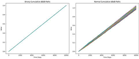
Left: selection of outcomes from random walk
Right: selection of outcomes from normal distribution (Brownian)

Integrating dBdB (=dt) over [0,1], increments = 100

Integrating dBdB (=dt) over [0,1], increments = 1000

Integrating dBdB (=dt) over [0,1], increments = 10000

Integrating a Sigmoid function w.r.t. dBdB (=dt) over [0,1], increments = 10000

Intuiting Stochastic Calculus in Python

Coding done in Python

Brownian motion on the real line is conceived as a limit of the random walk. A small enough step for a random walk is then taken to simulate brownian motion. Given a finite standard deviation, from the central limit theorem, the distribution from which we take each step gives the same limit.

In Ito integration, we often encounter dBdB = dt. When the distribution of the random walk is taken to be 1 at 1/2 and -1 at 1/2, then with any approximation, this exactly holds true. When given a normal distribution, we see that as we increase the number of increments to simulate, the stochastic integral becomes more and more precise, as the variance of the square of dB converges to 0 faster than the mean (note that the variance of the sum of independent distributions the sum of their variances, and therefore the integral converges as the increments go to zero).

Swapping Dwayne Johnson and my face.

Example of a case of mode collapse

Ground Truth simulated from Heat Equation
(alpha = 2)

Noise added

Data informed NN
(Sampled frames = 20, 30, ..., 100)
Final Prediction at frame 200

Conservation of Energy and Heat Equation
(Sampled frames = 20, 30, ..., 100)

Gathered and augmented data and trained a custom designed cycleGAN architecture.

Coding done in Python with Pytorch.

Investigated the use of physics informed neural networks to find the thermal diffusivity of a insulated uniform 2D surface given noisy simulated data and investigated predictability.

Coding done in python with Tensorflow

kalman filter.pdf (click to download)

Blockchain.pdf (click to download)

Investigated and implemented the Kalman filter for its use in stock trading. Wrote explanatory notes on the method.

Investigated the blockchain protocol and wrote extensive notes on the subject.

Investigated Automatic Differentiation algorithms and wrote a fully generalized python implementation for both forward and backward accumulation versions. Also wrote expository notes on the subject.

Backprop in neural networks is a particular type of backward accumulation autodiff method.

Plotting 500 assets from the S&P 500 between 60 day asset alpha with respect to its beta to its fractal dimension (Minkowski–Bouligand dimension).

Coding done in python with MatPlotLib